Relief unit and raster objects
Gerald H. Taranto
Mon 28, March, 2022
Source:vignettes/articles/ghp/scapesClassification_02_4_OBJ.Rmd
scapesClassification_02_4_OBJ.RmdLoad data
Libraries and data are loaded and processed as explained in format input data.
# LOAD LIBRARIES
library(scapesClassification)
library(terra)

# LOAD DATA
grd <- list.files(system.file("extdata", package = "scapesClassification"), full.names = T)
grd <- grd[grepl("\\.grd", grd)]
grd <- grd[!grepl("hillshade", grd)]
rstack <- rast(grd)

# COMPUTE ATTRIBUTE TABLE
atbl <- attTbl(rstack, var_names = c("bathymetry", "local_bpi", "regional_bpi", "slope"))

# COMPUTE NEIGHBORHOOD LIST
nbs <- ngbList(rstack, rNumb = TRUE, attTbl = atbl) # neighbors are identified by their row number in the attribute table
Class vector filters
We will also add to the attribute table the class vector of the island shelf unit (ISU) and the class vector of the peak cells so that they can be used to build classification rules.
# LOAD ISU CLASSIFICATION
ISU <- list.files(system.file("extdata", package = "scapesClassification"), full.names = T,
                  pattern = "ISU_Cells.RDS")

atbl$ISU <- readRDS(ISU)
atbl$ISU[!is.na(atbl$ISU)] <- 1 # Class 1 identifies all ISU cells

# LOAD PEAK CLASSIFICATION
PKS <- list.files(system.file("extdata", package = "scapesClassification"), full.names = T,
                  pattern = "PKS_Cells.RDS")
atbl$PKS <- readRDS(PKS)

head(atbl)
## Cell bathymetry local_bpi regional_bpi slope ISU PKS
## 1 1 -1718.056 -4 129 1.410384 NA NA
## 2 2 -1737.816 -3 107 2.021313 NA NA
## 3 3 -1755.392 -1 87 2.482018 NA NA
## 4 4 -1787.728 -16 52 3.149354 NA NA
## 5 5 -1819.800 -33 18 2.125063 NA NA
## 6 6 -1806.728 -7 28 1.895863 NA NAPlots
In the following example we will show how the class vectors of raster objects are computed. However, in order to improve the reading experience, the plots’ code is hidden. It can be accessed in the *.RMD file used to generate the html file.
The plotting procedure is to (i) convert a class vectors into a raster using the function cv.2.rast() and to (ii) visualize the raster using R or an external software. In our example we will use the R package terra to create static maps and the R packages mapview and leaflet to create interactive maps (note that mapview do not support terra raster objects yet, therefore, they have to be converted into raster raster objects before plotting).
Relief unit
The relief unit (RU) is composed of prominent seamounts, banks and ridges. In this article individual elements of the relief unit will be classified as distinct raster objects each characterized by a unique ID (Figure 1 and Figure 4). The set of all objects will define the relief unit of our working example.
RU objects
In this example, relief units objects will be identified in a sequence of classification steps using raster object functions (Figure 1). Our functions will perform the following tasks:
anchor.seed: identify all raster cells (i) on prominent relieves that are (ii) not ISU cells and that are (iii) in continuity with peak cells. It assigns a different ID to each non-continuous group of cell (Figure 1a).
rel.pi: compute the standardized relative position index (
rPI) of each raster object.pi.sgm: (i) segment raster objects at locations that have negative
rPIor local bpi values; (ii) remove small raster objects composed of less than 40 cells (Figure 1b).pi.add: add new raster objects composed of (i) cells that have local bpi values
>100and (ii) that do not border any other object (i.e. an object is added only if it is disjoint from other objects) (Figure 1c).cond.4.nofn: homogeneous growth of raster objects. At turns, each object adds contiguous cells having local or regional bpi values
>100(Figure 1d).
Additional information about the above functions is available at the following links: function documentation and object functions (article).
# 1. ANCHOR.SEED
# Tasks:
# Identify raster cells on prominent features in connection with peak cells
# that are not within island shelf units (ISU).
atbl$RO <- anchor.seed(atbl, nbs, rNumb = TRUE, silent = TRUE,

                       class = NULL, # A new ID is assigned to every
                                     # discrete group of cells...

                       cond.seed   = "PKS == 1", # ...in continuity with peak cells...

                       cond.growth = "regional_bpi >= 100", # ...that are on prominent features.

                       cond.filter = "regional_bpi >= 100 & is.na(ISU)") # Only consider non-ISU cells
                                                                         # on prominent features.

rRO1 <- cv.2.rast(rstack, atbl$RO) # store raster for plotting
#######################################################################################################

# 2. REL.PI
# Tasks:
# Compute the standardized relative position index (`rPI`) of each raster object.
atbl$rPI <- rel.pi(atbl, RO="RO", el="bathymetry")
#######################################################################################################

# 3. PI.SGM
# Tasks:
# (i) Segment large raster objects that have negative rPI or negative local bpi;
# (ii) Remove raster objects with less than 40 cells.
atbl$RO <- pi.sgm(atbl, nbs, rNumb = TRUE,
                  RO = "RO",
                  mainPI = "rPI",
                  secPI = "local_bpi",
                  cut.mPI = 0,
                  cut.sPI = 0,
                  min.N = 40)

rRO2 <- cv.2.rast(rstack, atbl$RO) # store raster for plotting
#######################################################################################################

# 4. PI.ADD
# Tasks:
# Add new raster objects composed of cells with local_bpi>100;
# An object is added only if it is disjoint from other objects,
# if it has more than 40 cells and if it is not within the ISU.
atbl$RO <- pi.add(atbl, nbs, rNumb = TRUE,
                  RO = "RO",
                  mainPI = "local_bpi",
                  add.mPI = 100,
                  min.N = 40,
                  cond.filter = "is.na(ISU)")

rRO3 <- cv.2.rast(rstack, atbl$RO) # store raster for plotting
#######################################################################################################

# 5. COND.4.NOFN (HGROWTH)
# Task:
# Homogeneous growth of raster objects;
# At turns, each raster object adds contiguous cells having
# regional or local BPI values > 100
IDs <- unique(atbl$RO)[!is.na(unique(atbl$RO))]

atbl$RO <- cond.4.nofn(atbl, nbs, rNumb = TRUE, classVector = atbl$RO,
                       nbs_of = IDs, class = NULL,
                       cond = "regional_bpi > 100 | local_bpi > 100",
                       hgrowth = TRUE)

rRO4 <- cv.2.rast(rstack, atbl$RO) # store raster for plotting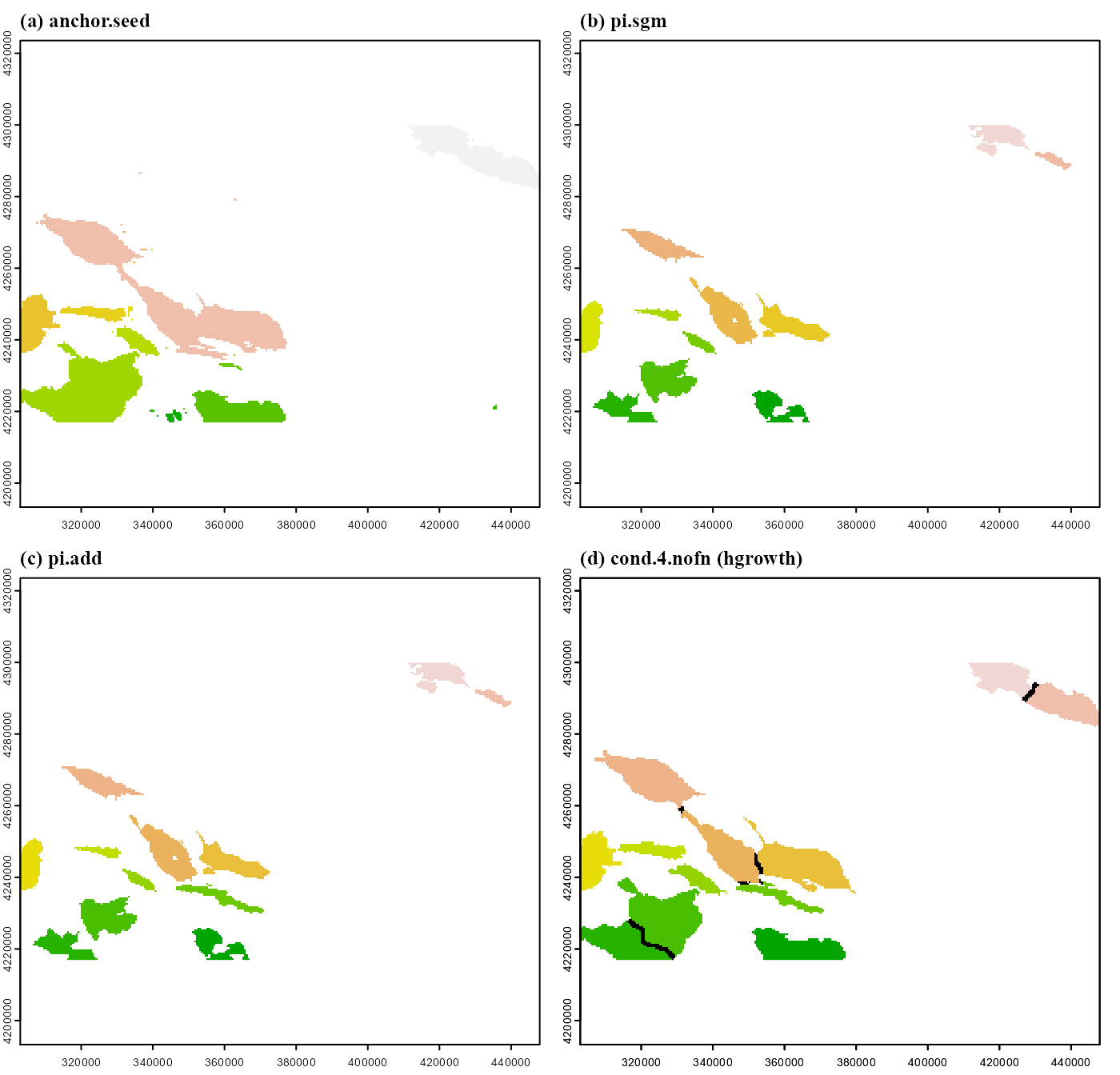
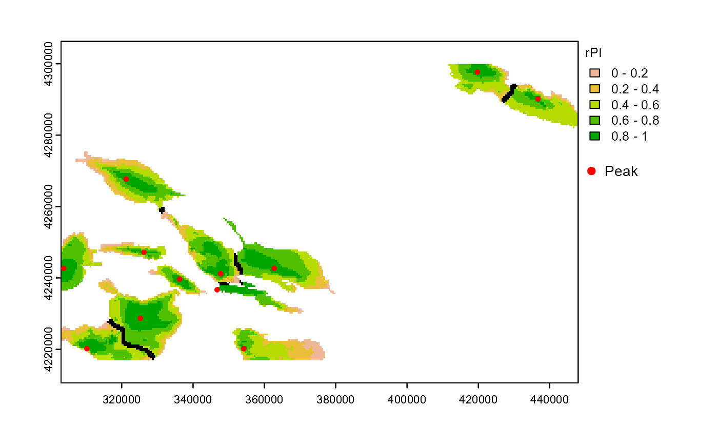
Relative position index
As we saw in the previous section, relative position indices are useful to segment and to identify raster objects. Another important quality of position indices is that they allow to visualize the depth distribution of individual objects and, thus, discern where summits and bases are (Figure 2).
Ridges
Ridge systems are an ecologically important component of relieves. In this section we will identify the distinct ridges existing within the relief unit. We will adopt a simple definition of what a ridge is:
They are within raster objects;
They have high local bpi values (
>100);They have a minimum of 20 cells.
The first two rules are implemented using anchor.seed, the last using pi.sgm (Figure 3).
# IDENTIFY RIDGES
atbl$RDG <- anchor.seed(atbl, nbs, rNumb = TRUE, silent = TRUE, class = NULL,
                        cond.seed   = "local_bpi > 100",
                        cond.growth = "local_bpi > 100",
                        cond.filter = "!is.na(RO)")

# REMOVE SMALL RIDGES
atbl$RDG <- pi.sgm(atbl, nbs, rNumb = TRUE, RO = "RDG", min.N = 20)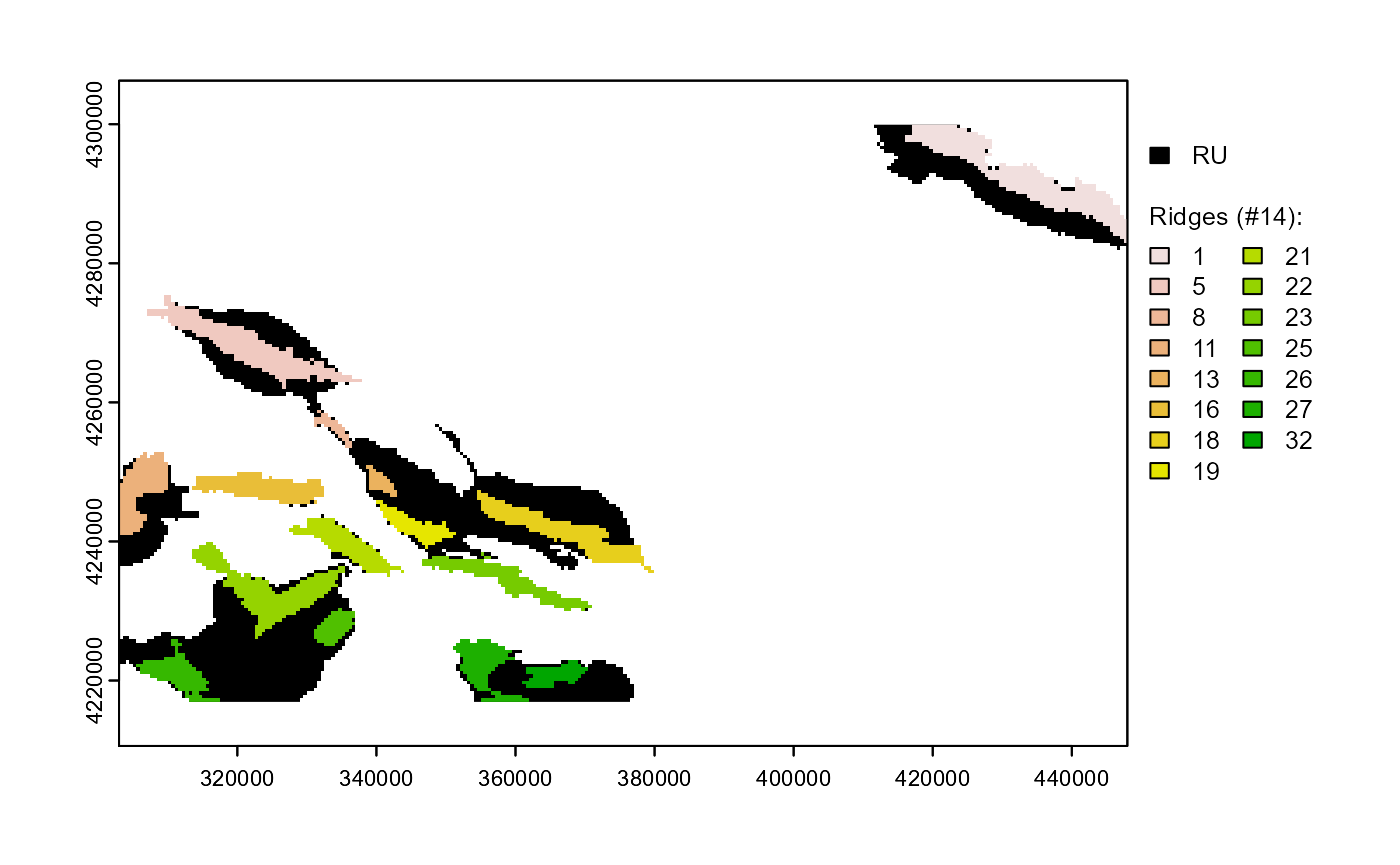
Data.table
The R package data.table provides an easy syntax to handle and transform groups within tables and facilitates the computation of group statistics. In the context of scapesClassification, it can be used to facilitate hierarchic classifications and to summarize raster object statistics.
As an example, we will first compute some simple statistics for each raster object: number of cells (N), average (avgD), maximum (maxD), minimum (minD) and standard deviation (sdD) of depth values. In addition, we will count the number of discrete ridges each object contains (nRDG) and the percentage of the object they cover (pRDG).
Finally we will rename raster object IDs based on the rank of minimum depth values: the raster object with the lowest minimum depth value will have ID = 1; the object with the highest minimum depth value will have the highest ID.
# DATA TABLE
library(data.table)

# CONVERT ATTRIBUTE TABLE TO ATTRIBUTE 'DATA' TABLE
atbl <- as.data.table(atbl)

# COMPUTE STATISTICS
RO_stat <- atbl[!is.na(RO),

                .(N = .N,
                  minD = round(max(bathymetry), 2),
                  avgD = round(mean(bathymetry), 2),
                  maxD = round(min(bathymetry), 2),
                  sdD = round(sd(bathymetry), 2),
                  nRDG = sum(!duplicated(RDG), na.rm = TRUE),
                  pRDG = round(sum(!is.na(RDG))/.N, 2)),

                by = "RO"]

# RENAME AND RANK RO IDs BY MIN. DEPTH
new_IDs <- RO_stat[, data.table::frankv(minD, order = -1L)]

atbl[!is.na(RO), RO := new_IDs[match(RO, RO_stat$RO)] ]
RO_stat[, RO := new_IDs][order(RO)][]
## RO N minD avgD maxD sdD nRDG pRDG
## 1: 1 1085 -164.33 -447.77 -990.34 166.59 3 0.39
## 2: 2 821 -194.38 -844.95 -1619.83 327.34 2 0.46
## 3: 3 643 -215.83 -439.85 -724.87 105.18 2 0.24
## 4: 4 934 -361.47 -748.36 -1491.84 208.84 2 0.32
## 5: 5 221 -361.54 -756.60 -1153.92 186.03 2 0.98
## 6: 6 203 -388.59 -637.19 -1010.62 143.62 2 0.91
## 7: 7 486 -407.62 -831.13 -1468.64 203.98 2 0.41
## 8: 8 669 -474.04 -635.18 -870.95 92.08 4 0.28
## 9: 9 627 -490.24 -1048.44 -1448.86 181.98 3 0.42
## 10: 10 452 -559.19 -802.79 -1279.67 144.86 2 0.45
## 11: 11 572 -719.49 -1129.49 -1604.93 138.88 2 0.54
## 12: 12 233 -778.42 -1019.78 -1600.48 201.87 2 0.90Interactive maps
Raster objects can be visualized as interactive maps using the R packages mapview and leaflet. Each object can be associated to a pop-up using the R package leafpop. The combined use of scapesClassification, data.table and interactive maps provides users with the capacity to highlight areas of interest, summarize raster object statistics and share the outcome.
As an example we will produce an interactive map of the relief unit objects with pop-up windows presenting the statistics computed with data.table (Figure 4).